
Description
Coursework for the Deep Learning Module. It involved building, training and tuning two types of latent space generative models. The first was a Convolutional VAE trained on MNIST and the second a DCGAN trained on CIFAR-10.
Details
| Skills: | Deep Learning VAE GAN Pytorch Python |
| Scope: | University |
| Date: | February 2024 |
Components
-
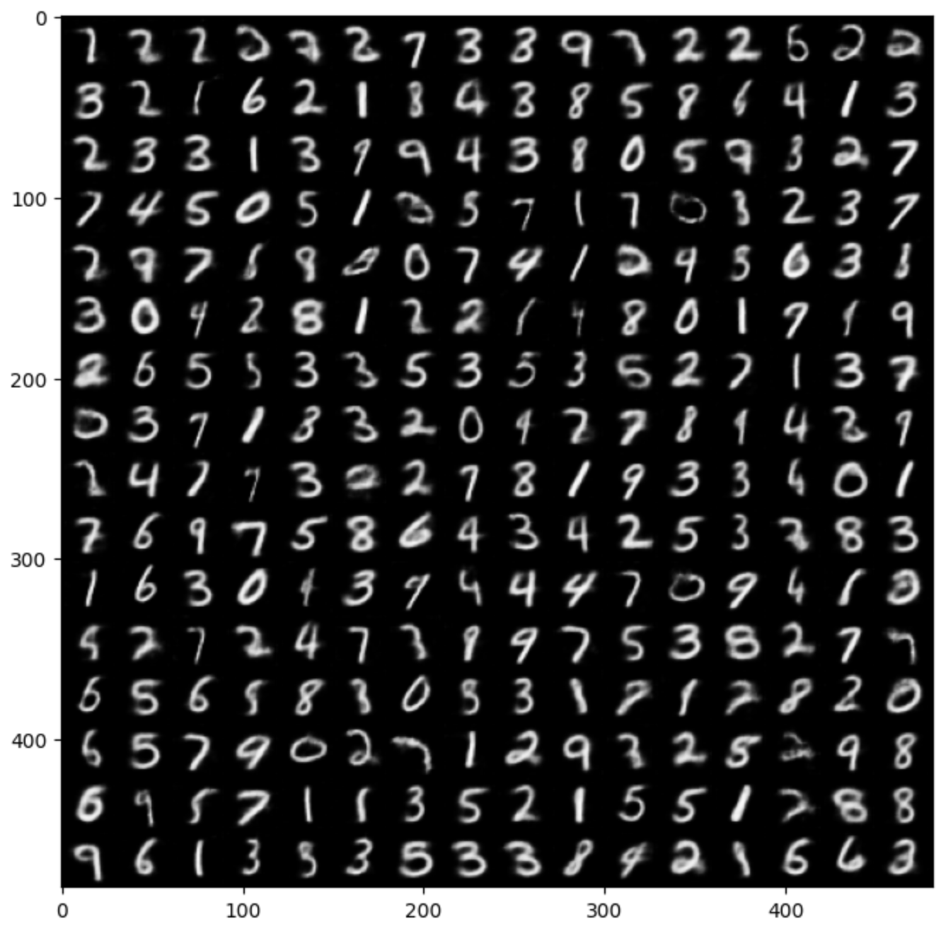
Variational Auto Encoder: The VAE had to be built from scratch, requiring extensive
research and testing to ensure a sufficient performance was achieved. Most of the design decisions
made were a result of repeated experimentation and testing:
- Cost Function: A reconstruction loss added to a KLD term for the distribution divergence from the prior, modified by a parameter beta. For the reconstruction loss there were two main options: the commonly used MSE, but also BCE with a Sigmoid activation (as MNIST uses only one channel). Extensive explorations were conducted using both options and very little difference was observed besides requiring different magnitudes of Beta. In the end, the MSE loss was settled on since it produced a more disentangled latent space for each image class (which could be seen in the TSNE embeddings). The KLD term was implemented using the analytical form with a Normal Gaussian Prior. This prior was chosen for two main reasons: Image generation and Latent Space Exploration. Using a Gaussian Normal helped with image generation as it ensured that the latent space representations of all the features were similar, meaning generation could involve simply filling the latent space with random samples from a Normal Gaussian which could then be passed through the decoder to generate images. The second is that the normal gaussian has a logvar and mean of zero, resulting in a number of network activations being driven to 0, promoting sparsity and disentangelement of the latent space.
- Structure: Additional explorations were made in regards to the architecture of the encoder and decoder. To reduce the number of parameters two downconvolution layers were used with stride 2, reducing the image size from 28x28 to 7x7, followed by two linear layers to bottleneck the forwards pass and encourage a good latent space representation; these layers were interspersed with batchnorms and leaky ReLU layers to increase convergence speed. The decoder was implemented as a reversed encoder.
-
Deep Convolutional Generative Adverserial Network: The GAN was built based on the model proposed by
Unsupervised Representation Learning with Deep Convolutional Generative
Adversarial Networks and tuned once again through testing different modifications:
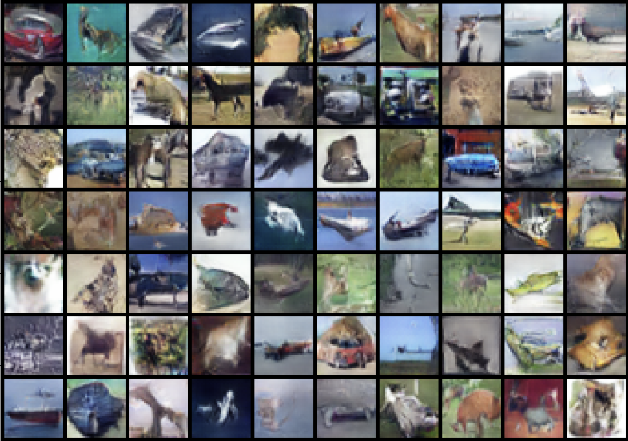
- Kernel Size: Performance was tested with different Kernel Sizes, 3x3 had very poor performance, producing images with strange colours and patterns. Kernels of 7x7, 9x9 and 11x11 generated images that appear similar to those created by the 5x5, though with seemingly fewer details or discernable shapes (possibly because many kernels act on each pixel causing some level of 'smoothing').
- Latent Space: Different latent space sizes were also explored, a size of 200 resulted in more diverse images, though with fewer discernable items; a size of 50 created less diverse and lower quality images, though with more distinction. Running the model with 75 seemed to capture the best of both worlds, producing images containing a larger array of diverse yet recognisable items.
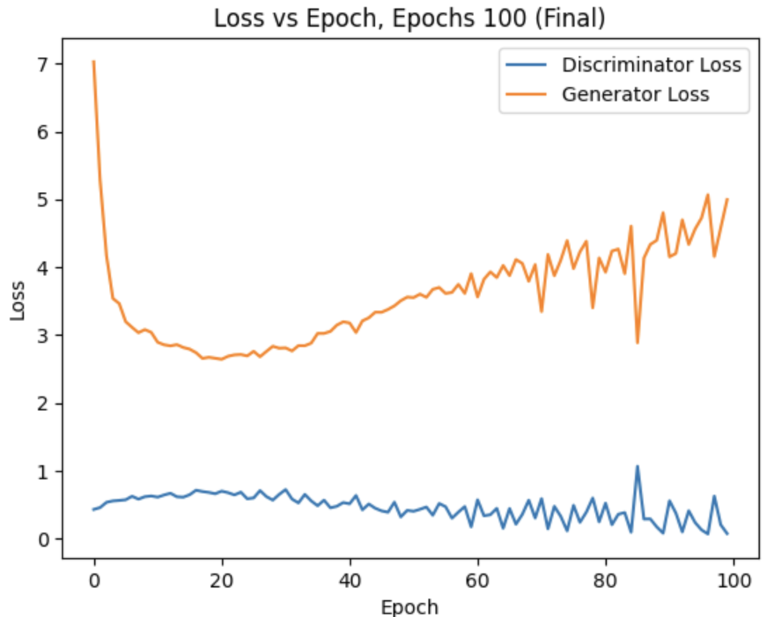
- Epochs When testing it was discovered that models with loss curves that remain at an 'equilibrium' of sort for a number of epochs tended to perform better when simply trained for longer. As the network is adverserial, the loss is no real indication of overall performance as the Generator and Discriminator can improve at the same rate. The network was trained for 20, 50 and 100 epochs, demonstrating overall improved image generation after longer training. Analysing loss curves showed that going for too long resulted in overfitting as the Discriminator slowly learned all the images in the dataset, naturally making it discriminate more efficiently.